---

Viewing and Analyzing Trace Data

Because Instruments lets you gather data from multiple instruments simultaneously, the amount of data available to you can quickly get overwhelming. Fortunately, Instruments devotes much of its interface to organizing and displaying data in ways that help you analyze and navigate that data. Understanding the different areas of your trace document window is essential to spotting trends and finding potential problem areas.

Every trace document includes the following interface elements:

• The Track pane

• The Detail pane

• The Extended Detail pane

• The Run Browser

Each of these elements show you the exact same data in your trace document; they just show it in very different ways, ranging from high-level overviews to detailed information about each data point. The idea is to give you different ways to visualize your data. You can view the high-level data to look for general trends, and then look at the detailed data to find out exactly what is happening in your code and formulate ideas on how to fix potential issues.

In addition to the user interface options, many instruments can be configured to present their data in several different ways. You can use these configuration options during the analysis phase to get fresh perspectives on the gathered data.

In this chapter, you learn how to use the information provided to you by Instruments and how you can modify the way that information is presented it to suit your workflow needs.

In this section:

Tools for Viewing Data
Analysis Techniques

Tools for Viewing Data

The following sections describe key elements of the Instruments user interface and how you use those elements to view trace data.

The Track Pane

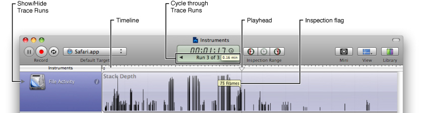
The most prominent portion of a trace document window is the track pane. The track pane occupies the area immediately to the right of the instruments pane. This pane presents a high-level, graphical view of the data gathered by each instrument. You use this pane to examine the data from each instrument and to select the areas you want to investigate further.

The graphical nature of the track pane makes it easier to spot trends and potential problem areas in your program. For example, a spike in a memory usage graph indicates a place where your program is allocating more memory than usual. This spike might be normal, or it might indicate that your code is creating more objects or memory buffers than you had anticipated in this location. An instrument such as the Spin Monitor instrument can also point out places where your application becomes unresponsive. If the graph for the Spin Monitor is relatively empty, you know that your application is being responsive, but if the graph is not empty, you might want to examine why that is.

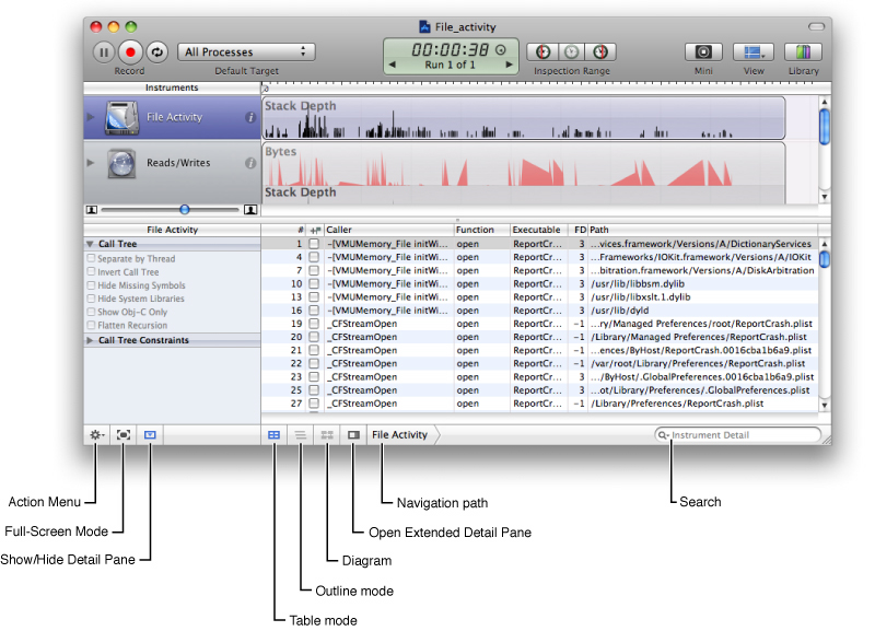
Figure 5-1 shows a sample trace document and calls out the basic features of the track pane. You use the timeline at the top of the pane to select where you want to investigate. Clicking in the timeline moves the playhead to that location and displays a set of inspection flags, which summarize the information for each instrument at that location. Clicking in the timeline also focuses the information in the Detail pane on the surrounding data points; see “The Detail Pane.”

Although each instrument is different, nearly all of them offer options for changing the way data in the track pane is displayed. In addition, many instruments can be configured to display multiple sets of data in their track pane. Both features give you the option to display the data in a way that makes sense for your program.

The sections that follow provide more information about the track pane and how you configure it.

Viewing Trace Runs

Each time you click the Record button in a trace document, Instruments starts gathering data for the target processes. Rather than append the new data to any existing data, Instruments creates a new trace run to store that data. A trace run constitutes all of the data gathered between the time you clicked the Record button and stopped gathering data by clicking the Stop button. By default, Instruments displays only the most recent trace run in the track pane, but you can view data from previous trace runs in one of two ways:

• Use the Time/Run control in the toolbar to select which trace run you want to view.

• Click the disclosure triangle next to an instrument to display the data for all trace runs for that instrument.

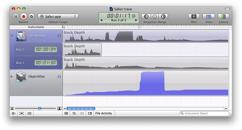
Figure 5-2 shows an instrument that has been expanded to show multiple trace runs. In this example, several trace runs have been collected, each of which was generated from a slightly different set of events. You might gather multiple trace runs when you are trying to reproduce a problem that does not occur every time, creating new trace runs until the problem surfaces. If you want to compare multiple trace runs using the exact same set of events, however, you need to create a user interface track, a process that is described in “Working with a User Interface Track.”

When you save a trace document, Instruments normally discards the data from all runs except the one that is currently selected. It does this to keep the size of your trace documents from becoming too large. If you want to save all trace runs for your documents, go to the General tab of the Instruments preferences and uncheck the Save Current Run Only option.

Displaying Multiple Data Sets for an Instrument

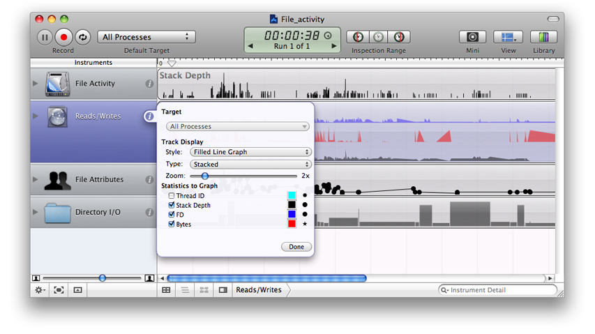
Some instruments are capable of displaying multiple streams of data inside their corresponding track pane. You can configure which streams of data are displayed using the instrument inspector, as shown in Figure 5-3. The Statistics to Graph section lists all of the integer-based data values gathered by the instrument. Selecting the checkboxes in that section adds the corresponding statistics to the track pane.

For information about the data gathered by each instrument, see “Built-in Instruments.”

Changing the Display Style of a Track

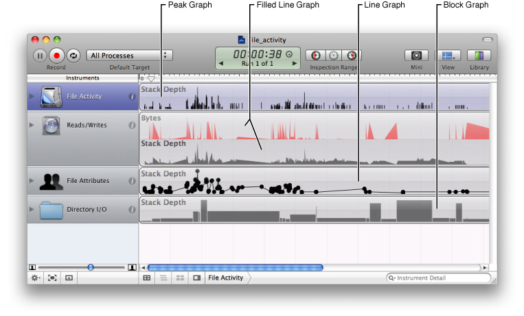
Instruments provides several different styles for graphing data in the track pane. Most instruments choose a style that makes the most sense for the type of data they are displaying. You can change the selected style for an instrument using the Style pop-up menu in the instrument’s inspector. Figure 5-4 shows several of the styles.

Zooming in the Track Pane

Instruments supports zooming in and out on track pane data along both the vertical and the horizontal axes.

• To change the horizontal (time) scale, use the slider control below the instruments pane.

• To change the vertical (amplitude or volume) scale, select an instrument and do one of the following:

  • Open the instrument’s inspector and use the Zoom slider there.

  • Select the View > Increase Deck Size menu item to increase the zoom factor.

  • Select the View > Decrease Deck Size menu item to decrease the zoom factor.

For horizontal zooming, Instruments expands or contracts the track pane around the current playhead position. If you set the playhead to a particular point before zooming, you can zoom in or out on the data under that point.

The Detail Pane

After you identify a potential problem area in the track pane, you use the Detail pane to examine the data in that area. The Detail pane displays the data associated with the current trace run for the selected instrument. Instruments displays only one instrument at a time in the Detail pane, so you must select different instruments to see different sets of details.

Different instruments display different types of data in the Detail pane. Figure 5-5 shows the Detail pane associated with the File Activity instrument, which records information related to specific file system routines. The Detail pane in this case displays the function or method that called the file system routine, the file descriptor that was used, and the path to the file that was accessed. For information about what each instrument displays in the Detail pane, see “Built-in Instruments.”

To open or close the Detail pane, do one of the following:

• Choose View > Detail.

• Click the View button in the toolbar and select Detail from the pull-down menu.

• Click the Toggle Detail Pane button at the bottom left of the trace document window, next to the Full Screen mode button.

• Select Detail from the Action menu at the bottom of the Instruments window.

Changing the Display Style of the Detail Pane

For some instruments, you can display the data in the Detail pane using more than one format. The Detail pane supports the following formatting modes:

• Table mode displays a flat list of aggregated sample data.

• Outline mode displays a hierarchical list of samples, typically organized using stack trace or process information.

• Diagram mode displays a list of the individual samples

To view an instrument’s data using one of these formats, click the appropriate mode button along the bottom of the Detail pane (see Figure 5-5). Which modes an instrument supports depends on the type of data gathered by that instrument. For example, the Sample instrument supports only table and outline modes, but the Network Activity instrument supports all three modes.

When displaying data in Outline mode, you can use disclosure triangles in the appropriate rows to dive further down into the corresponding hierarchy. Clicking a disclosure triangle expands or closes just the given row. To expand both the row and all of its children, hold down the Option key while clicking on a disclosure triangle.

Sorting in the Detail Pane

You can sort the information displayed in the Detail pane according to the data in a particular column. To do so, click the appropriate column header. The columns in the Detail pane differ with each instrument.

Searching in the Detail Pane

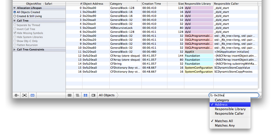
You can type a string in the search field in the lower-right corner below the Detail pane to narrow down the list of information displayed in the Detail pane. By default, Instruments applies the specified search string against all of the data recorded by the instrument. With some instruments, however, you can refine the scope of your search even further. For example, use the ObjectAlloc instrument to apply the search string against specific subsets of the instrument data, such as the library or routine that created the memory block. You can even search for objects at a specific memory address.

The filter scoping criteria varies from instrument to instrument. To specify the desired scope, click the magnifying glass in the search field and choose from the available options. Figure 5-6 shows the search options for the ObjectAlloc instrument.

Viewing Data for a Range of Time

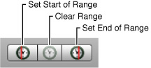
Although zooming in on a particular event in the track pane lets you see what happened at a specific time, you may also be interested in seeing the data collected over a range of time. You use the Inspection Range control (shown in Figure 5-7) to focus on the data collected in a specific time range.

To mark a time range for inspection, do the following:

1. Set the start of the range.

   1. Drag the playhead to the desired starting point in the track pane.

   2. Click the leftmost button in the Inspection Range control.

2. Set the end of the range.

   1. Drag the playhead to the desired endpoint in the track pane.

   2. Click the rightmost button in the Inspection Range control.

Instruments highlights the contents of the track pane that fall within the range that you specified. When you set the starting point for a range, Instruments automatically selects everything from the starting point to the end of the current trace run. If you set the endpoint first, Instruments selects everything from the beginning of the trace run to the specified endpoint.

You can also set an inspection range by holding the Option key and clicking and dragging in the track pane of the desired instrument. Clicking and dragging makes the instrument under the mouse the active instrument (if it is not already) and sets the range using the mouse-down and mouse-up points.

When you set a time range, Instruments filters the contents of the Detail pane, showing data collected only within the specified range. You can quickly narrow down the large amount of information collected by Instruments and see only the events that occurred over a certain period of time.

To clear an inspection range, click the button in the center of the Inspection Range control.

The Extended Detail Pane

For some instruments, the Extended Detail pane shows additional information about the item currently selected in the Detail pane. To open or close the Extended Detail pane, do one of the following:

• Choose View > Extended Detail.

• Click the Toggle Extended Detail Pane button at the bottom of the Instruments window, next to the navigation bar.

• Click the View button and choose Extended Detail from the pull-down menu.

• Select Extended Detail from the action menu at the bottom of the Instruments window.

The Extended Detail pane usually includes a description of the probe or event that was recorded, a stack trace, and the time when the information was recorded. Not all instruments display this information, however. Some instruments may not provide any extended details, and others may provide other information in this pane. For information about what a particular instrument displays in this pane, see the instrument descriptions in “Built-in Instruments.”

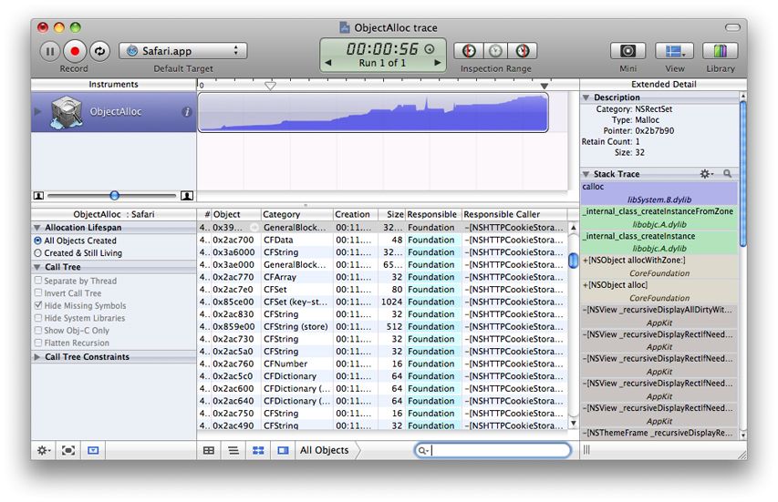
Figure 5-8 shows the Extended Detail pane for the ObjectAlloc instrument. In this example, the instrument displays information about the type of memory that was allocated, including its type, pointer information, and size.

For instruments that display stack trace information in the Extended Detail pane, double-clicking an entry for which you have source code opens the source file in Xcode. You can also configure the information shown in the stack trace using the Action menu at the top of that section. Clicking and holding the Action menu icon displays a menu from which you can enable or disable the options in Table 5-1.

In addition, if you have an Xcode project with the source code for the symbols listed in a stack trace, you can double-click a symbol name in the Extended Detail pane to launch Xcode and jump to the relevant source code.

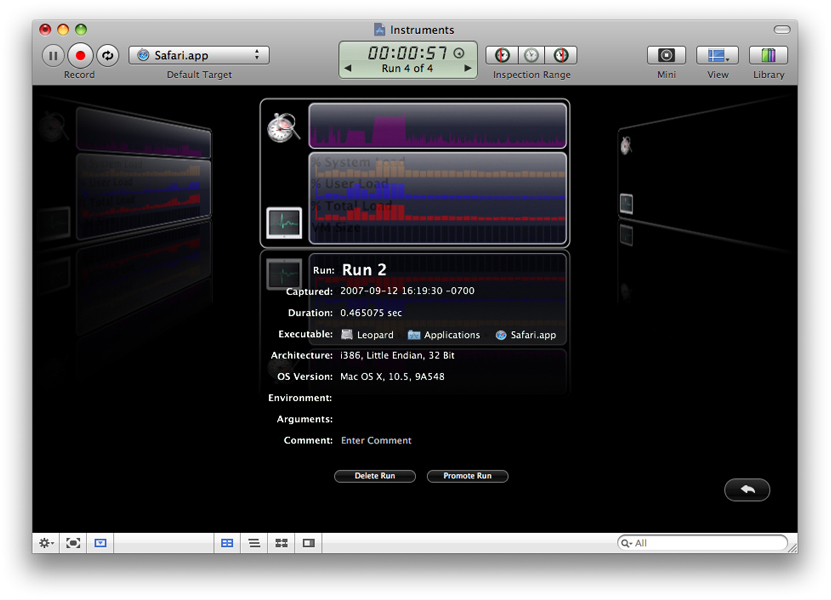
The Run Browser

The Run Browser is a way to view and manage previous runs quickly. If your trace document contains numerous runs, you can use this mode to scan those runs for the one you want and promote it to the top of the list. You can also delete runs and add comments to runs from this view.

To open the Run Browser, select View > Run Browser.

“The Run Browser” shows the Run Browser view in Instruments. Clicking views on either side of the selected view scrolls the new view into focus. To enter a comment for a view, double click the text in the Comment field to make it editable. To exit the Run Browser view, click the return arrow button in the bottom-right portion of the window.

Analysis Techniques

Gathering and viewing trace data is easy. Analyzing that data and locating potential problems is hard. It is this latter task where the art of performance tuning and debugging comes into play. Recognizing patterns in the massive amounts of data gathered by performance tools can be daunting, even for experienced developers. This is where having the right tools (and knowing how to use them) makes all the difference. The instruments that come with the Instruments application provide many different options for organizing and filtering trace data. The following sections describe some of the behaviors and options available for specific instruments and how you use those instruments to identify issues in your code.

Analyzing Data with the Sampler Instrument

The Sampler instrument is a tool for performing a statistical analysis on a running application. Performing a statistical analysis involves stopping an application at regular intervals and recording information about what was executing at that moment in time. For each thread, the Sampler instrument records information about the functions and methods currently on the stack, including the name of the function or method and the module that owns it. After gathering the data, it coalesces the call stack information from the individual samples to form a master call tree for the application. This tree shows all of the execution paths that were seen during sampling and how many times each one was seen.

The advantage of statistical sampling is that it is a lightweight and convenient way to find out what your application is doing over a period of time. The technique can be used on any application without specially instrumenting the code, and it usually offers a reasonably accurate picture of your application’s runtime behavior.

The disadvantage of statistical sampling, however, is that it does not give you a 100% accurate picture of what your application is doing. Because it only takes snapshots of the call stack at periodic intervals, the Sampler instrument does not record an exact history of all of the functions and methods that were executed. With typical sampling intervals on the order of 1 to 10 milliseconds, it is possible for a lot of functions and methods to be called between samples. Despite this seemingly inaccurate picture, statistical sampling does work for most applications when enough samples are gathered. Over time, the distortions caused by the sampling interval tend to smooth out as more samples are gathered. As a result, statistical sampling is still a good way to gather information about your application quickly and without too much effort.

Analyzing the Call Stack Data

The purpose of the Sampler instrument is to show you where your application is spending its time. It does this by showing you which functions were called and how often they were called.

The place to start in the Sampler tool is the Track pane. By default, the track pane graphs the maximum call stack depth for all the threads of the application. (You can also change this graph to show the CPU load instead.) Because it offers a visual approach, the Track pane can help you spot trends in your code. Repeated patterns can indicate similar code paths being executed. The shape of different sections can also give some indication as to what they were doing. By clicking in an interesting area, you can then begin analyzing the data at that area using the Detail pane.

The Detail pane is where you do a more in-depth analysis of your code. The Detail pane supports both the Table and Outline viewing modes. Table mode presents you with the time-ordered list of samples. You can use this list to see what code was executing at a given point in your application. In Outline mode, you are presented with the sample data organized by call stack. From this view, you can look at each execution branch of each thread and see which ones have unusually large numbers of samples. Expanding each thread lets you see the individual methods and functions and the number of samples gathered for each one. To expand an entire hierarchy all at once, hold down the Option key while clicking the disclosure triangle.

In addition to starting at a thread’s main routine and searching for heavy branches, you can also invert the call tree to start at the leaf nodes and see which methods and functions were called most often. Inverting the call tree can help quickly identify methods and functions that are perhaps being used too frequently. You can then expand the tree from these leaf nodes to find out who called that method or function and how often. While doing this, it is often helpful to display the number of milliseconds the given method or function spent running so that you can correlate the number of samples with the actual amount of time that function used.

The Extended Detail pane provides you with additional views of the sample data. In Table mode, the pane displays the data gathered by the selected sample, which includes the stack traces for all threads running when the sample was taken. In Outline mode, it shows the deepest stack trace containing the selected method or function.

Filtering the Contents of the Detail Pane

Table 5-2 lists the high-level configuration options you can apply to samples gathered with the Sampler instrument. You use these options to focus your analysis on the events that occurred at a particular time or that involve a particular portion of your code.

The Call Tree configuration options offer several ways to trim down the call tree without removing any sample data. When you hide or flatten a set of symbols, Sampler applies the samples for those symbols to the calling function or method. This lets you remove any symbols that you cannot control and focus on your own code and how much time it took to execute.

Alternatively, the Call Tree Constraints actually remove sets of samples from the view to let you focus on code paths that meet specific criteria. For example, you might use a time-based constraint to focus on code paths that took at least 100 milliseconds to run.

When applying an instrument’s configuration options, do not forget that you can also constrain the sample data based on when those samples were gathered. The Inspection Range control in each trace document lets you view the data from a specific set of sample points. This feature works in combination with all of the instrument’s other configuration options. For more information on how to use the Inspection Range control, see “Viewing Data for a Range of Time.”

Analyzing Data with the ObjectAlloc Instrument

The ObjectAlloc instrument is a tool for tracking all of the memory allocations made by an application. You can then use that information to identify memory allocation patterns in your application and identify places where your application is using memory inefficiently. The ObjectAlloc instrument provides data trimming and pruning facilities that are equal to or better than the former ObjectAlloc application. Because it is integrated with the Instruments environment, you can also use the instrument to correlate your application’s memory behavior with other types of behavior.

Because it tracks memory allocations over the life of an application, you must launch your application from Instruments so that the ObjectAlloc instrument can gather the data it needs. At launch time, the ObjectAlloc instrument uses existing hooks in the system to record information about allocation and deallocation events in your application, whether those events originated with the standard system malloc routines or your own custom malloc library. As data flows in, the instrument updates its displays in real time to show you how memory is being allocated.

The ObjectAlloc instrument works with applications that use the standard malloc functions (such as malloc, calloc, and free) but also works with garbage collected applications. In the latter case, the collector still issues free calls for GC-aware memory. The ObjectAlloc instrument also works with routines built on top of malloc, including the memory allocation routines in both Core Foundation and Cocoa.

Analyzing the Object Allocation Data

The purpose of the ObjectAlloc instrument is to show you how your application is using memory. Memory is an important system resource that you should use wisely. Each memory allocation has both an immediate cost and a potential long-term cost. The immediate cost is the time it takes to allocate the memory, which could involve creating new virtual memory pages and mapping them into physical memory. It could also involve writing out stale memory pages to disk. Long term, keeping blocks resident in physical memory can trigger additional paging in the system, which as with all paging operations can seriously hamper performance.

Like all tools, the place to start in the ObjectAlloc tool is the Track pane. In its default configuration, the Track pane graphs the net amount of memory currently in use by your application. Using the instrument’s inspector, you can change this view to show the allocation density, which shows you where the memory allocations occurred, or you can display the stack depth. The allocation density graph lets you see how frequently memory allocations occurred throughout your program. Spikes in the allocation density can indicate potential bottlenecks that you might want to mitigate by preallocating some blocks or being more lazy about other blocks.

Regardless of which display options you set using the inspector, the Track pane displays the allocations for all types of objects by default. To focus on a specific subset of memory allocations, you can use the Detail pane to configure which objects you want to include in the Track pane’s graph. To focus on a particular object type or block size, open the Detail pane and set it to Table mode. In this mode, the Detail pane sorts memory allocations by object type or size. The Graph column contains checkboxes for selecting which objects you want to graph. Disabling the All Allocations checkbox (which is enabled by default) and enabling the checkbox for another object type updates the Track pane accordingly. If you enable multiple checkboxes, the ObjectAlloc instrument layers the graphs on top of each other using different colors.

The Detail pane (while it is in Table mode) displays other useful information to help you spot potential allocation issues. The net versus overall allocations column of the table shows a histogram of the currently active objects and the total number that were ever created. As the ratio of net allocations to overall allocations shrinks, the color of the histogram bar changes. Blue histogram bars represent a reasonable ratio while colors shifted towards the red spectrum represent lower ratios that might warrant some investigation.

Although Table mode is very useful for getting an overall picture of your allocations, the Detail pane takes advantage of all three viewing modes. Table 5-3 describes the information presented in each mode and how you might use that mode to look for problems.

The Extended Detail pane for the ObjectAlloc instrument primarily displays stack trace information for the selected allocation event. For some allocation events, this pane also displays descriptive information about the event, including the type and size of the event and the object retain count (if any). This information is there to help you locate the allocation event in your code.

Tracking Reference Counting Events

When you add the ObjectAlloc instrument to your document, the instrument is initially configured to record only memory allocation and deallocation events. By default, it does not record reference counting events, such as CFRetain and CFRelease calls. The reason is that recording reference counting events adds significant overhead to the data gathering process and is not needed in all situations. If your code is leaking memory, however, you might want to configure the ObjectAlloc instrument to record these events as part of your effort to track down the leaks. In particular, you can look for any mismatched retain and release events to see if an object is still retained when the last reference to it is removed.

To enable the gathering of reference counting events, open the inspector for the ObjectAlloc instrument and enable the “Record reference counts” option.

Filtering the Contents of the Detail Pane

Table 5-4 lists the high-level configuration options you can apply to memory events recorded by the ObjectAlloc instrument. You use these options to focus your analysis on the events that occurred at a particular time or that involve a particular portion of your code. All of these options apply only when viewing data in Outline and Diagram modes. In Table mode, the ObjectAlloc instrument displays the history of all allocations.

When applying an instrument’s configuration options, do not forget that you can also constrain the sample data based on when those samples were gathered. The Inspection Range control in each trace document lets you view the data from a specific set of sample points. This feature works in combination with all of the instrument’s other configuration options. For more information on how to use the Inspection Range control, see “Viewing Data for a Range of Time.”

Looking for Memory Leaks

The Leaks instrument provides leak-detection capabilities identical to those in the leaks command-line tool. This instrument analyzes the in-use memory blocks of your application looking for blocks that are no longer referenced by your code. Unreferenced blocks are deemed “leaks” because they cannot be freed by your application and continue to occupy memory space until the user quits the application.

Eliminating memory leaks from your application is an important step toward improving your application’s reliability. This is especially true for applications that are designed to run for long periods of time. Leaks increase your application’s overall memory footprint, which can lead to paging. Applications that continue to leak memory may even find themselves unable to complete an operation because they cannot allocate the necessary memory. In extreme cases, the application may become so impaired that it crashes.

The Leaks instrument records all allocation events that occur in your application and then periodically searches the application’s writable memory, registers, and stack for references to any active memory blocks. If it does not find a reference to a block in one of these places, it reports the buffer as a leak and displays the relevant information in the Detail pane.

In the Detail pane, you can view leaked memory blocks using Table and Outline modes. In Table mode, Instruments displays the complete list of leaked blocks, sorted by size. Clicking the follow link button next to a memory address shows the allocation history for memory blocks at that address, ultimately culminating in an allocation event without a matching free event. Selecting one of these allocation events displays the stack trace for that event in the Extended Detail pane along with general information about the memory block. In Outline mode, the Leaks instrument displays leaks organized by call tree. You can use this mode to find out how many leaks are in a specific branch of your code and how much memory was leaked by that branch. Selecting a branch displays the deepest code path for that branch in the Extended Detail pane.

Table 5-5 lists the configuration options for the Leaks instrument. Many of these options affect how leaks looks for information, but some affect how leaked buffers are reported.

For information about the leaks command-line tool, see leaks man page.

Analyzing Core Data Applications

For applications that use Core Data to manage their underlying data model, Instruments provides several Core Data–related instruments to analyze potential performance issues. These instruments give you insight into the events happening behind the scenes in Core Data and may help you identify places where your your application is not fetching or saving data efficiently. Table 5-6 lists the provided instruments and how you might use each one.

The Core Data template creates a new trace document containing the Core Data Fetches, Core Data Cache Misses, and Core Data Saves instruments. This template is the recommended starting point for analyzing your Core Data applications.

For more information about tuning a Core Data application, see Core Data Programming Guide.

---